Lecture #2: Mathematical Modeling of Control Systems
2-1 Introduction
In studying Control Systems, we need to be able to model dynamic systems in mathematical terms and analyze their dynamic characteristics. We can represent the dynamic system by using a set of differential equations. Keep in mind that there is not one single set of differential equations that govern a system, there may be others that are valid depending on the perspective. We can obtain these differential equations using fundamental laws that govern a particular system (ie. Newton's Laws for Mechanical Systems, Kirchhoff's Laws for Electrical Systems, ect.). Obtaining and deriving these equations are the most important part of the entire analysis of control systems!
Throughout all of our material, we will assume causality, by which the current output (at t=0) depends on the past input (at t<0) but does not depend on the future input (a t>0).
Throughout all of our material, we will assume causality, by which the current output (at t=0) depends on the past input (at t<0) but does not depend on the future input (a t>0).
- Mathematical Models
- Models may take many forms. Depending on the system one model may be better suited than another. For example, the use of state space representation (as we will discuss soon) is suited for optimal control problems. While transfer functions may be more convenient for transient response ore frequency response analysis of a single-input, or for single output linear time-invariant systems.
- Simplicity vs. Accuracy
- You will find that we must take a compromise between the simplicity of the model and the accuracy of the model. It is often necessary to ignore certain inherent physical properties of a system. For example, if a mathematical model using ordinary differential equations (known as a linear-lumped model) is used, it is always necessary to ignore certain non-linearities. The effect of these ignored properties should have small change to the response, and still provide good agreement between the experimental model and the physical model.
- Keep in mind that ignoring these parameters may have a valid output at low frequencies, but at higher frequencies the ignoring could throw off the response completely.
- Linear Systems
- A system is considered linear iff the principle of superposition applies
- ie. The simultaneous application of two different forcing functions is equal to the sum of the two individual responses
- This can make it simple to find the response to several inputs just by treating one input at a time and summing them all up individually
- A system is considered linear iff the principle of superposition applies
- Linear Time-Invariant Systems and Linear Time-Varying Systems
- A differential equation is considered Linear if the coefficients are constants or functions of the independent variable
- Linear Time-Invariant Systems are made of differential equations that have constant coefficients
- Linear Time-Varying Systems are made of differential equations that have coefficients that are functions of time
- A differential equation is considered Linear if the coefficients are constants or functions of the independent variable
2-2 Transfer Function and Impulse Response Function
Transfer Functions for linear, time-invariant, differential equation systems are defined as the ratio of the Laplace Transform of the output to the Laplace of the input under the assumption that all initial conditions are zero.
Consider the linear time-invariant system defined by the following differential equation:
Consider the linear time-invariant system defined by the following differential equation:
Where y is the output of the system, and x is the input. The transfer function of this system is the ratio seen below:
Using Transfer Functions we can represent system dynamics by algebraic equations in the s domain. The order of the system is said to be the highest order of s which as seen in the equation above is represented by n, which we consider to be an "nth-order system".
Important Notes about Transfer Functions:
Convolution Integral
Let's consider that we have a given transfer function as defined by G(s):
Important Notes about Transfer Functions:
- The applicability of Transfer Function is limited to only linear, time-invariant, differential equation systems.
- The transfer function is a mathematical model that is an operational method of expressing the differential equation that relates the output variable to the input variable
- The transfer function is a property of a system itself, which is independent of the magnitude and nature of the input specifically
- The transfer function of many physically different systems can be identical
- If the transfer function of a system is known, the output or response can be studied for various forms of input to better understand the system
- If the transfer function is unknown it may be experimentally established by introducing known inputs and studying the output of the system
Convolution Integral
Let's consider that we have a given transfer function as defined by G(s):
From this equation we can backtrack from the Laplace Domain to the time domain. Note that multiplication in the complex domain is equivalent to convolution in the time domain, so the inverse Laplace Transform of the equation above looks like this:
Impulse-Response Function
When we say "Impulse-Response" we are saying that we will be using a unit-impulse function. The important thing to know is that the Laplace Transform of a unit-impulse function is unity (ie. X(s) = 1 ). Thus we end up having the output of our system equal to the transfer function of our system as shown:
When we say "Impulse-Response" we are saying that we will be using a unit-impulse function. The important thing to know is that the Laplace Transform of a unit-impulse function is unity (ie. X(s) = 1 ). Thus we end up having the output of our system equal to the transfer function of our system as shown:
From this extraction we can then use the convolution integral we talked about above to take the inverse Laplace Transform of the complex function to find what the transfer function g(t) is in the time domain, g(t) is also called the weighting function of the system.
It is hence possible to obtain complete information about the system dynamics by exciting it with an impulse input and measuring the response. While the ability to create impulse function in real life do not exist, pulse inputs with a very short duration can be considered an impulse.
2-3 Automatic Control Systems
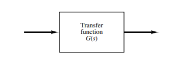
A complete control system may be comprised of multiple components. In order to show the functions performed by each component, in control engineering we utilize what are known as block diagrams. A block diagram of a system is a pictorial representation of the functions performed by each component and the flow of signals. These diagrams have the advantage over mathematical models of being able to indicate more realistically the signal flow of the system. The figure below indicates a single element of the block diagram, you can see the arrow point into the block being the input signal, and the arrow pointing out being the output signal.
Note that the dimensions of the output signal from the block is the dimensions of the input signal multiplied by the dimension of the transfer function block.
Summing Points
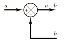
As seen in the picture below, a circle with a cross is the symbol that indicates a summing operation. The plus or minus sign at each arrow head inidcates whether the signal is to be added or subtracted to yield the output.
As seen in the picture below, a circle with a cross is the symbol that indicates a summing operation. The plus or minus sign at each arrow head inidcates whether the signal is to be added or subtracted to yield the output.
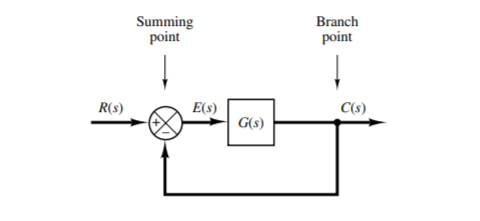
A branch point differs from summing point in which it is a point from which the signal from a block goes concurrently to other blocks or summing points.
Block Diagram of a Closed-Loop System
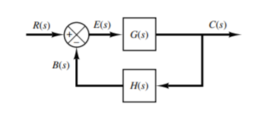
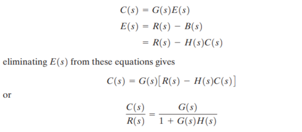
As we had talked about before, a closed loop system is created by feeding the output of the system back into a transfer function which is then compared to a reference value which is then fed back into the system as an input. As seen from the diagram below, output C(s) is fed back to the summing point after being multiplied by H(s) where it is then compared to the reference R(s). It is a reasonable question to ask why we have H(s) and not directly just feed C(s) into the summing point, this is because often the dimension is different. For example C(s) may be temperature in Celsius, but most electrical systems in order to use this temperature as a feedback input must first convert it into a voltage using a thermistor/thermocouple. H(s) represents the transfer function of the sensor that is responsible for the conversion from temperature to voltage.
From the system above we can come up with the transfer function quite simply by relating the output C(s) to the input R(s) by using the following relations:
Open-Loop Transfer Function and Feed-forward Transfer Function
By examining the picture provided by the Closed-Loop System, you can see that the ratio of the feedback B(s) to the actuating error signal E(s) is known as the open-loop transfer function
Another important transfer function and what makes for the basis of Open-Loop system is known as the feed-forward transfer function, which can be seen from the closed loop system diagram by the ratio of C(s) to the actuating error signal E(s).
Automatic Controllers
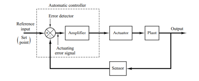
An automatic controller is simply defined to compare the actual value of the plan output with the reference input (aka desired value), determines the deviation, and produces a control signal that will reduce the deviation to zero or to a small value. The manner in which the controller produces the control signal is called the control action.
An automatic controller is simply defined to compare the actual value of the plan output with the reference input (aka desired value), determines the deviation, and produces a control signal that will reduce the deviation to zero or to a small value. The manner in which the controller produces the control signal is called the control action.
Classifications of Industrial Controllers
- Two-Position / On-Off Controllers / Bang-Bang Controllers
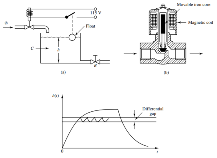
- These controllers have only two fixed positions which are in many cases simply on or off, they seek to make the error between the output and the reference value zero by switching on if the error is too low, and switching off if the error is too high (could be vise versa)
- Some of these kinds of controller do not simply just have a fixed value in which they will switch on or off if higher than or lower than the specified value. Instead they provide a minimum and maximum bound in which the output must reside within known as a differential gap
- You can reduce the high peak oscillations in the differential gap by decreasing the range of the gap
- Proportional Control Action
- Controllers with this implementation relate the output of the controller u(t) to the actuating error signal e(t) my multiplying with a constant Kp, which is known as the proportional gain
- Integral Controller Action
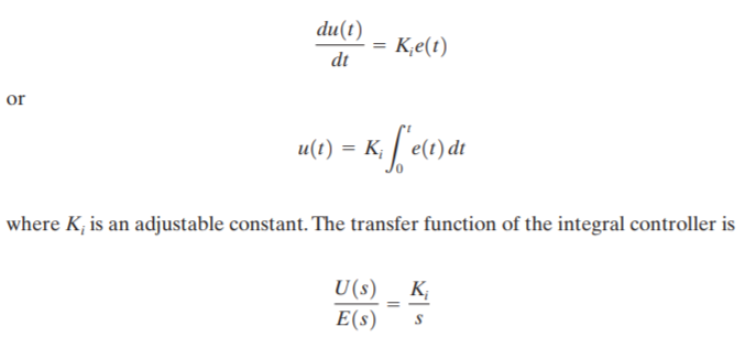
- Controllers with this implementation have the controller output u(t) change at a rate proportional to the actuating error signal e(t) such that:
- Proportional-Plus-Integral Control Action
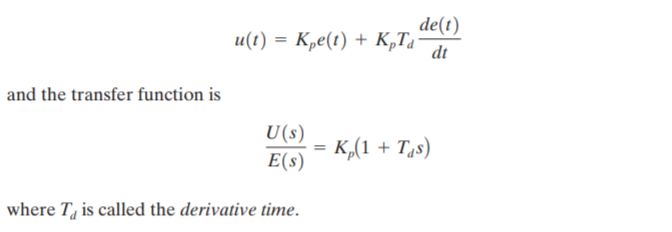
- Proportional-Plus-Derivative Control Action
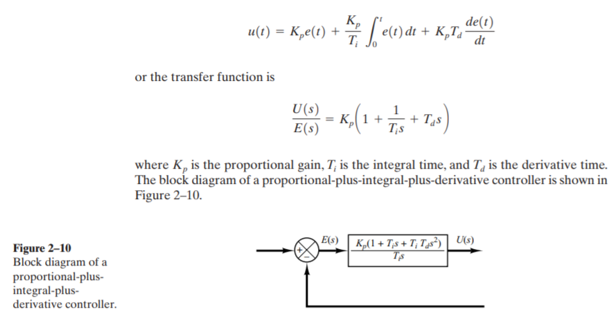
- Proportional-Plus-Integral-Plus-Derivative Control Action
- This combination has the advantage of each of the three control actions. The equation of a control with this combined action is given by:
Procedures for Drawing a Block Diagram
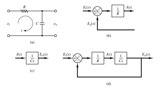
To draw a block diagram for a system, first write each of the equations that describe the dynamic behavior of each component. Then take the Laplace transform of each of these equations. Then you can assemble these pieces into a block diagram. Here is an example:
To draw a block diagram for a system, first write each of the equations that describe the dynamic behavior of each component. Then take the Laplace transform of each of these equations. Then you can assemble these pieces into a block diagram. Here is an example:
Block Diagrams Reduction
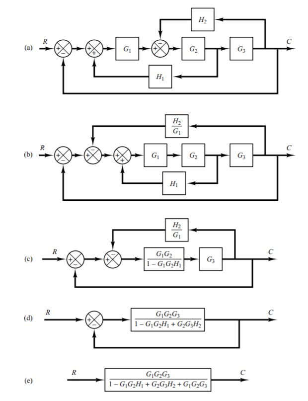
When blocks are in series with one another they can be simplified into a single block by multiplying the two transfer functions. If however the diagram is more complex with multiple feedback portions a step by step rearrangement is necessary for simplification, as seen in the example below. You can see that by my multiplying or dividing the the transfer functions we can move where the arrow points in the system.
When blocks are in series with one another they can be simplified into a single block by multiplying the two transfer functions. If however the diagram is more complex with multiple feedback portions a step by step rearrangement is necessary for simplification, as seen in the example below. You can see that by my multiplying or dividing the the transfer functions we can move where the arrow points in the system.
2-4 Modeling in State Space
Modern Control Theory vs. Conventional Control Theory
These two versions of control theory are often contrasted with one another.
These two versions of control theory are often contrasted with one another.
- Modern Control Theory
- Applicable to Multiple-input, Multiple-output systems which may be nonlinear, time invariant or time varying
- Is a time-domain and frequency approach
- Conventional Control Theory
- Applicable to linear, time-invariant single-input, single-output systems
- Is a complex frequency-domain approach
- State
- The state of a system is the smallest set of variables, known as the state variables such that the knowledge of these variables at time T0, together with the knowledge of the input for t > T0, then it can completely determine the behavior of the system for any time t > T0
- State Variable
- These are the individual variables that determine the state of the dynamic system.
- State Vector
- If n state variables are needed to completely determine the behavior of a given system, then these n state variables can be considered the n components of a vector x , such a vector is known as the state vector
- State Space
- The n-dimensional space whose coordinate access consist of the x1 axis, ..., xn axis. Any state can be represented by a point in the state space
- State-Space Equations
- In State Space Analysis we are interested in 3 types of variables in modeling dynamic systems:
- Input Variables
- Output Variables
- State Variables
- Keep in mind that the state space representation of a system is not unique, there may be multiple representations for a single system, but the number of state variables will be constant
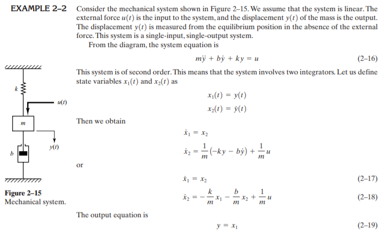
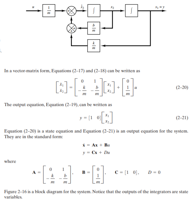
- Dynamic systems must involve elements that memorize the values of the input, integrators in a continuous time system serve as memory devices. Thus, outputs of integrators serve as the state variables
- The number of state variables to completely define the dynamics of a system is equal to the number of integrators involved in the system
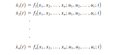
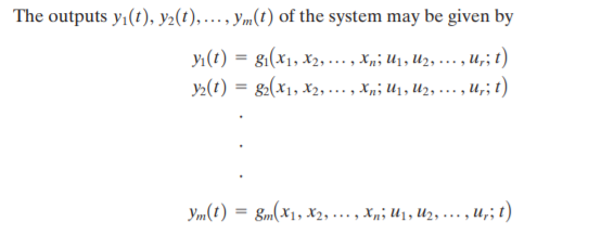
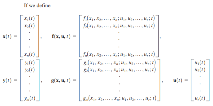
- Assume that a multiple-input, multiple-output system involves n integrators. Assume there are r inputs: u1(t), u2(t), ... , ur(t), and m outputs: y1(t), y2(t), ... , ym(t). Define n outputs of the integrators as state variables: x1(t), x2(t), ... , xn(t). Then the system my be described as:
- In State Space Analysis we are interested in 3 types of variables in modeling dynamic systems:
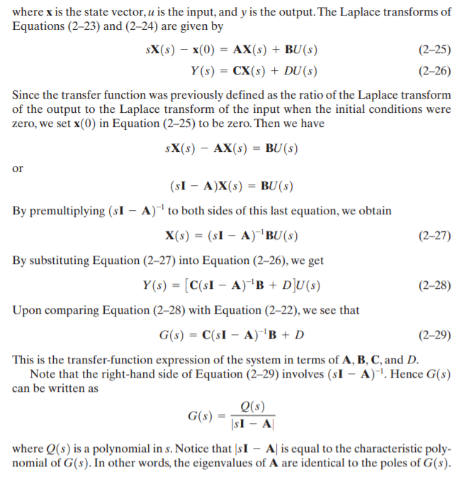
By combining the equations above, we can simplify ẋ(t) and y(t)
If we linearize the equations above about the operating state we get the following state equations:
- A(t) is the State Matrix
- B(t) is the Input Matrix
- C(t) is the Output Matrix
- D(t) is the Direct Transmission Matrix
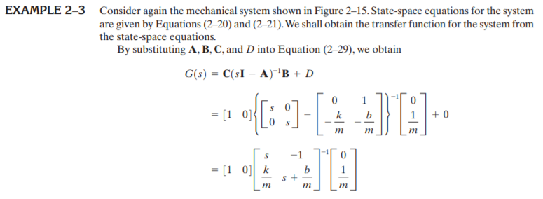
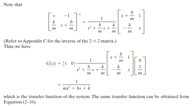
Correlation Between Transfer Functions and State-Space Equations
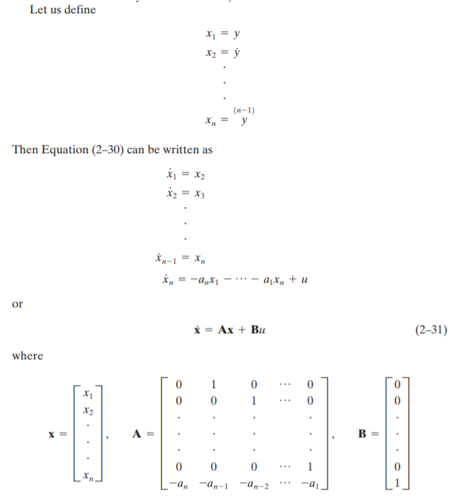
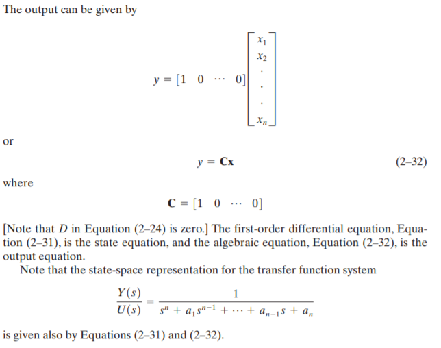
This is very similar to the approach we took above, but with an n-th order differential equation, so the state vector is size n.
- State-Space Representation of nth-Order Systems of Linear Differential Equations in which the Forcing Function Does Not Involve Derivative Terms.
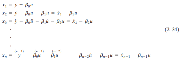
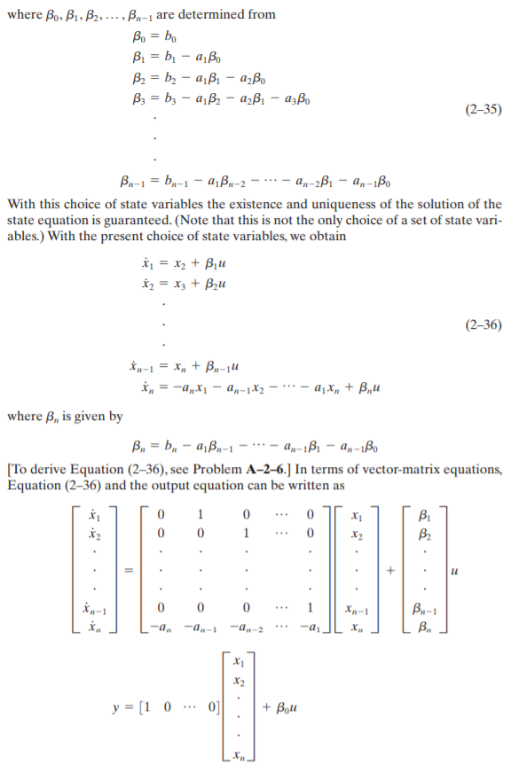
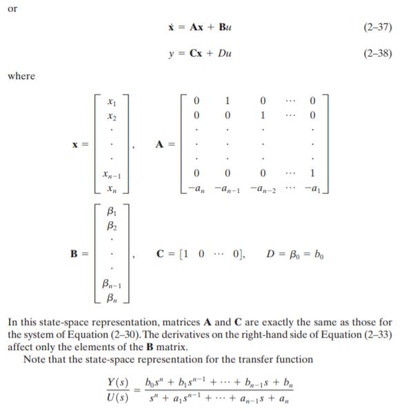
- State-Space Representation of nth-Order Systems of Linear Differential Equations in which the Forcing Function Involves Derivative Terms.


