A Recap of the Science and Math
Calculus
Lots of people dread the idea that calculus concepts will be used in hybrid design, but most of the calculus will really just be done by calculators. However, understanding how we will be using calculus to analyse the trajectory of rockets will be our main focus. Let's first start with Differentiation. In high school physics they taught us that acceleration was represented this way:
Lots of people dread the idea that calculus concepts will be used in hybrid design, but most of the calculus will really just be done by calculators. However, understanding how we will be using calculus to analyse the trajectory of rockets will be our main focus. Let's first start with Differentiation. In high school physics they taught us that acceleration was represented this way:
a = ΔV / Δt
where the Greek letter Δ represents "a finite change in". (ΔV happens a lot in rocketry)
No one in high school every really bothered to tell you that this is just a special base of differential calculus, the specialization being that this acceleration is constant over the measured time interval (meaning that for this to be correct, the velocity would need to be linearly changing). So if the velocity-versus-time graph were to be some exponential graph, then this method of calculating the acceleration would be invalid. If this was the case that the acceleration wasn't constant due to the velocity changing non-linearly over time, then we might rather be interested in the instantaneous acceleration at a particular time. We get this by using a infinitesimally small time interval for our Δt (but not exactly zero). Thus, in differential calculus we use the following equation:
No one in high school every really bothered to tell you that this is just a special base of differential calculus, the specialization being that this acceleration is constant over the measured time interval (meaning that for this to be correct, the velocity would need to be linearly changing). So if the velocity-versus-time graph were to be some exponential graph, then this method of calculating the acceleration would be invalid. If this was the case that the acceleration wasn't constant due to the velocity changing non-linearly over time, then we might rather be interested in the instantaneous acceleration at a particular time. We get this by using a infinitesimally small time interval for our Δt (but not exactly zero). Thus, in differential calculus we use the following equation:
a = dV / dt or a = d/ dt (v)
where d signifies a "very small change in". In Physics we would read this as "the time rate of change of velocity is equal to acceleration". One thing to note, is that the notation of d/dt was invented by a mathematician named Leibniz, but Newton would use a notation known as flexion notation where to denote the same thing he would put a dot above the variable. In rocketry we use both notations.
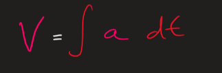
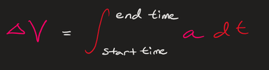
Newton also needed to create a reverse process to Differentiation known as Integration, in this way we could use the acceleration to calculate the change in velocity. Again, high school physics gave us a specialized equation that assumed acceleration was constant over the time interval.
Newton also needed to create a reverse process to Differentiation known as Integration, in this way we could use the acceleration to calculate the change in velocity. Again, high school physics gave us a specialized equation that assumed acceleration was constant over the time interval.
|
|
The curly line denotes integration. In Physics we would read this as "Velocity is the time integral of time". If you are looking for an instantaneous velocity value you can use the equation on the left which to find the equation for velocity based on time, then plug in the time value. If on the other hand you are trying to calculate the change in velocity over a specified period of time, you can use the bounded integration equation as shown on the right, specifying the start time and end time.
The value of this bounded integral is equal to the area under the curve within the bounded interval. We can approximate this value by using the Riemann sum equations.
The value of this bounded integral is equal to the area under the curve within the bounded interval. We can approximate this value by using the Riemann sum equations.
Forces
sadasm
sadasm
Weight and Mass
sadasm
sadasm
The Rocket Principle
sadasm
sadasm
Newton's Laws
sadasm
sadasm
The Kinetic Theory of Gasses
sadasm
sadasm
Temperature
sadasm
sadasm
The Mole
sadasm
sadasm
The Ideal Gas Law: Pressure, Temperature, and Density
sadasm
sadasm
Mass Continuity and Mass Flux
sadasm
sadasm
Energy
sadasm
sadasm
Mixture
sadasm
sadasm
Types of Rocket Engines
sadasm
sadasm
The Atmosphere
sadasm
sadasm
A Suborbital Trajectory
sadasm
sadasm