Lecture #1: Introduction to Control Systems
Automatic Control is an integral field of engineering and has many fundamental concepts that form the essence of control of Space-Vehicles, Robotic Systems, Modern Manufacturing Systems, and any Industrial Operations.
1-1 Introduction
Brief Review of Historical Developments of Control Theories and Practices
One of the most fundamental and what we consider to be the first example of an automatic control system is James Watt's 18th century Centrifugal Governor which provided speed control to the vehicle (We will talk a bit more about this later on). It was Watt's work that paved the pay for further discoveries by Minorsky, Hazen, and Nyquist.
- Minorsky who in 1922 implemented some automatic controllers for steering a ship and showed how the stability of a system could be determined from the differential equations that govern the system.
- Nyquist in 1932 who discovered a relatively simple method for determining the stability of a closed system based on the open loop response to a system based on steady-state sinusoidal inputs.
- Hazen in 1934 introduced the term "Servo-mechanics" for position control systems.
- Bode in the 1940's developed the Bode Diagram method which made it possible for engineers to design linear closed systems that satisfied performance requirements.
- Ziegler and Nichols suggested rules for the tuning of PID controllers in the early 1940's and introduced the Ziegler-Nichols Tuning Rules
- 1960-1980 the developments in computing allow for multiple input multiple output systems be solved much faster, and Optimal Control of both deterministic and stochastic systems was created
- 1980-1990 Modern Control Theory Centers on Robust Control
- Robust Control is done to compensate for the fact that a system's stability is sensitive to the error between the actual system and its model, and thus Robust control is focus on setting up a possible error range and as long as the model is in that range, it will be stable.
Definitions
Let's cover some basic terminologies, as not to get confused later on!
Let's cover some basic terminologies, as not to get confused later on!
- Controlled Variable: Is the quantity or condition that is measured on controlled
- Control Signal/Manipulated Variable: is the quantity of condition that is varied by the controller (This is usually the output)
- Control: means measuring the controlled variable and applying a Control Signal to correct/limit deviation
- Plant: Is supposed to be the piece of equipment we are trying to control (ie. mechanical device, electrical component, ect.)
- System: a Combination of components that act together and perform a certain objective
- Disturbances: A signal that tends to adversely affect the value of the output of a system
- Feedback Control: Refers to in the presence of disturbances will reduces the differences between the output and a reference input based on the difference.
1-2 Examples of Control Systems
|
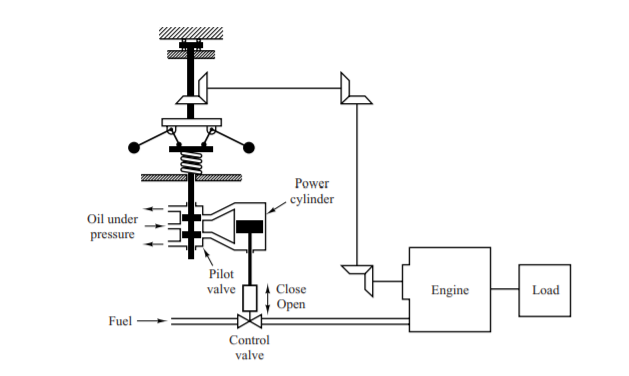
The image on the left is known as James Watt's Speed Governor for an engine. The amount of fuel is adjusted according to the difference between the desired and actual engine speeds.
Here are the sequence of steps:
|
|
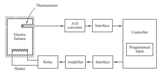
Shown on the left is a diagram outlining how an Electric Furnace's Temperature Control System operates. The system utilizes a thermometer to measure the temperature. The controller detects if the reading is above the desired value it will turn off the relay allowing more heat to build up. However, if the controller detects if the reading is lower than the desired value, then it will turn on the relay allowing for more heating to happen.
|
Robust Control System [DON'T WORRY ABOUT THIS UNTIL LATER LECTURES]
Robust Control is a very realistic form of control, in these lectures we will be using a model of the plant that we deem to be exactly representative of the system with zero uncertainty, we know however in real life this is not the case.
The first step to designing any Control System is to obtain a mathematical model of the Control Object(Plant). Regardless of the model you choose to use to model your plant, it will have some error compared to the reality of the model (this should be expected). In order to proceed with your design while knowing this, it is important to assume from the start that the mathematical model and the actual plant has an uncertainty or error. Following this type of design is known as Robust Control.
G'(s) = G(s)*[ 1 + Δ(s) ] or G'(s) = G(s) + Δ(s)
Ok, as if we didn't already have enough terms to understand, here are some more. Don't worry they are pretty basic!
Here are the parameters the govern the stability and performance of a Robust Control System:
Robust Control is a very realistic form of control, in these lectures we will be using a model of the plant that we deem to be exactly representative of the system with zero uncertainty, we know however in real life this is not the case.
The first step to designing any Control System is to obtain a mathematical model of the Control Object(Plant). Regardless of the model you choose to use to model your plant, it will have some error compared to the reality of the model (this should be expected). In order to proceed with your design while knowing this, it is important to assume from the start that the mathematical model and the actual plant has an uncertainty or error. Following this type of design is known as Robust Control.
- G'(s) = "The Actual Plant Model with an uncertainty (Δ)"
- G(s) = "The Nominal Plant Model to be used for designing the control system"
G'(s) = G(s)*[ 1 + Δ(s) ] or G'(s) = G(s) + Δ(s)
- W(s) = "Is a scalar transfer function that we will use to represent the uncertainty"
- || Δ(s) ||inf < ||W(s)||inf = maximum value of W(jw) between 0 and infinity
- This means that the scalar transfer function we are using the represent the uncertainty will always be greater than the uncertainty
Ok, as if we didn't already have enough terms to understand, here are some more. Don't worry they are pretty basic!
- K(s) = "The Transfer Function of the Controller"
- G(s) = "The Transfer Function of the Model"
Here are the parameters the govern the stability and performance of a Robust Control System:
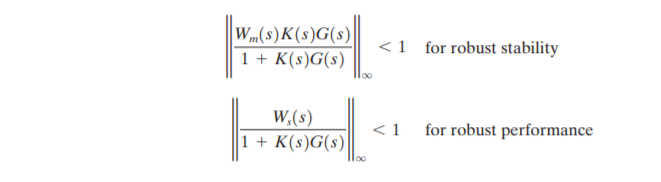
- Robust Stability: Means that the controller K(s) guarantees internal stability of all systems that belong to a group of systems that include the system with the actual plant
- Robust Performance: Means that the specified performance is satisfied in all systems that belong to the group
1-3 Closed-Loop Control vs. Open-Loop Control
- Feedback Control System: Is any system that maintains a relationship between the output and the reference input by comparing them and using the difference as a means of control
- Closed Loop Control Systems
- In these systems the actuating error signal, which is the difference between the input and the feedback signal (which may be the output itself or a function of the output signal)is fed into a controller as to reduce the error and bring the output of the system to a desired value.
- Implies the use of feedback to reduce system error
- Example: Temperature Control System
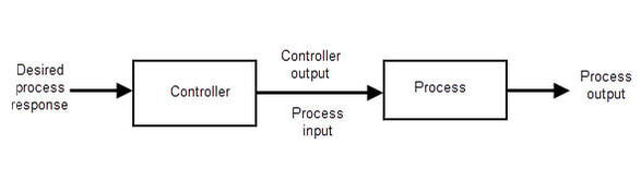
- Open Loop Control Systems
- In these systems the output has no effect on the control action
- The output is neither measured or compared
- These systems have fixed operating conditions, so as a result the accuracy of the system depends on calibration
- In the presence of disturbances the control system will be unable to perform
- Example: Traffic Lights or Washing Machine
Closed Loop vs. Open Loop
Closed Loop
|
Open Loop
|
1-4 Design and Compensation of Control Systems
- Compensation: is the modification of the system dynamics in order to satisfy the given specifications
- Our approaches to designing control and compensation systems is by using Root-Locus Approach, frequency-response approach, PID, and the state space approach. (We will discuss these in later lectures)
- Performance Specifications: Requirements imposed on the control system
- These relate to the accuracy, stability, and speed of response
- May be given in the form of:
- Transient response requirements (such as maximum overshoot and settling time in step response)
- Steady State Terms (such as steady state error in the ramp input)
- Frequency Response Terms
- System Compensation
- The first step in adjusting the system for satisfactory performance is by setting the gain. However, the adjustment of the gain may not be enough to meet specifications
- Increasing the gain will increase the steady state performance, but will result in poor stability or even instability
- We must then modify the structure or add in additional devices to redesign the system to meet specifications
- A device inserted into a system for this purpose is known as a compensator, which compensates for deficient performance of the original system
- The first step in adjusting the system for satisfactory performance is by setting the gain. However, the adjustment of the gain may not be enough to meet specifications
- Design Procedures
- Create Mathematical Model of the control system and adjust parameters for the compensator
- Check the system performance with each adjustment of the parameters (Most time consuming part, try to use MATLAB)
- Construct Open-loop system prototype
- Test Stability of the Open-loop system
- If stable, then close the loop and test performance of the now Closed-loop system
- There will almost always be some deviations that your model did not account for, you will need to adjust your compensation parameters to correct for that